DeePTB-E3: Bulk Silicon

DeePTB supports training an E3-equalvariant model to predict DFT Hamiltonian, density and overlap matrix under LCAO basis. Here, cubic-phase bulk silicon has been chosen as a quick start example.

Silicon is a chemical element; it has the symbol Si and atomic number 14. It is a hard, brittle crystalline solid with a blue-grey metallic lustre, and is a tetravalent metalloid and semiconductor (Shut up). The prepared files are located in:

deeptb/examples/e3/
|-- data
|   |-- Si64.0
|   |   |-- atomic_numbers.dat
|   |   |-- basis.dat
|   |   |-- cell.dat
|   |   |-- hamiltonians.h5
|   |   |-- kpoints.npy
|   |   |-- overlaps.h5
|   |   |-- pbc.dat
|   |   `-- positions.dat
|   `-- info.json
`-- input.json

We prepared one frame of silicon cubic bulk structure as an example. The data was computed using DFT software ABACUS, with an LCAO basis set containing 1 s and 1 p orbital. We now have an info.json file like:

{
        "nframes": 1,
        "pos_type": "cart",
        "pbc": true, # same as [true, true, true]
}

The input_short.json file contains the least number of parameters that are required to start training the DeePTB-E3 model, we list some important parameters:

"common_options": {
    "basis": {
        "Si": "1s1p"
    },
    "device": "cpu",
    "overlap": true
}

In common_options, here are the essential parameters. The basis should align with the DFT calculation, so 1 s and 1 p orbital would result in a 1s1p basis. The cutoff radius for the orbital is 7au, which means the largest bond would be less than 14 au. Therefore, the r_max, which equals to the maximum bond length, should be set as 7.4. The device can either be cpu or cuda, but we highly recommend using cuda if GPU is available. The overlap tag controls whether to fit the overlap matrix together. Benefitting from our parameterization, the fitting overlap only brings negligible costs, but is very convenient when using the model.

Here comes the model_options:

"model_options": {
    "embedding": {
        "method": "slem",
        "r_max": {
            "Si": 7.4
        },
        "irreps_hidden": "32x0e+32x1o+16x2e",
        "n_layers": 3,
        "avg_num_neighbors": 51,
        "tp_radial_emb": true
    },
    "prediction":{
        "method": "e3tb",
        "neurons": [64,64]
    }
}

The model_options contains embedding and prediction parts, denoting the construction of representation for equivariant features, and arranging and rescaling the features into quantum operators sub-blocks such as Hamiltonian, density and overlap matrix.

In embedding, the method supports slem and lem for now, where slem has a strictly localized dependency, which has better transferability and data efficiency, while lem has an adjustable semi-local dependency, which has better representation capacity, but would require a little more data. r_max should align with the one defined in info.json.

For irreps_hidden, this parameter defines the size of the hidden equivariant irreducible representation, which decides most of the power of the model. There are certain rules to define this param. But for quick usage, we provide a tool to do basis analysis to extract essential irreps.

In [1]: from dptb.data import OrbitalMapper

In [2]: idp = OrbitalMapper(basis={"Si": "1s1p"})

In [3]: idp.get_irreps_ess()
Out[3]: 2x0e+1x1o+1x2e

This is the number of independent irreps contains in the basis. Irreps configured should be multiple times of this essential irreps. The number can varies with a pretty large freedom, but the all the types, for example (“0e”, “1o”, “2e”) here, should be included for all. We usually take a descending order starts from “32”, “64”, or “128” for the first “0e” and decay by half for latter high order irreps. For general rules of the irreps, user can read the advance topics in the doc, but for now, you are safe to ignore!

In prediction, we should use the e3tb method to require the model output features using DeePTB-E3 format. The neurons are defined for a simple MLP to predict the slater-koster-like parameters for predicting the overlap matrix, for which [64,64] is usually fine.

Now everything is prepared! We can using the following command and we can train the first model:

cd deeptb/examples/e3
dptb train ./input_short.json -o ./e3_silicon

Here -o indicate the output directory. During the fitting procedure, we can see the loss curve of hBN is decrease consistently. When finished, we get the fitting results in folders e3_silicon.

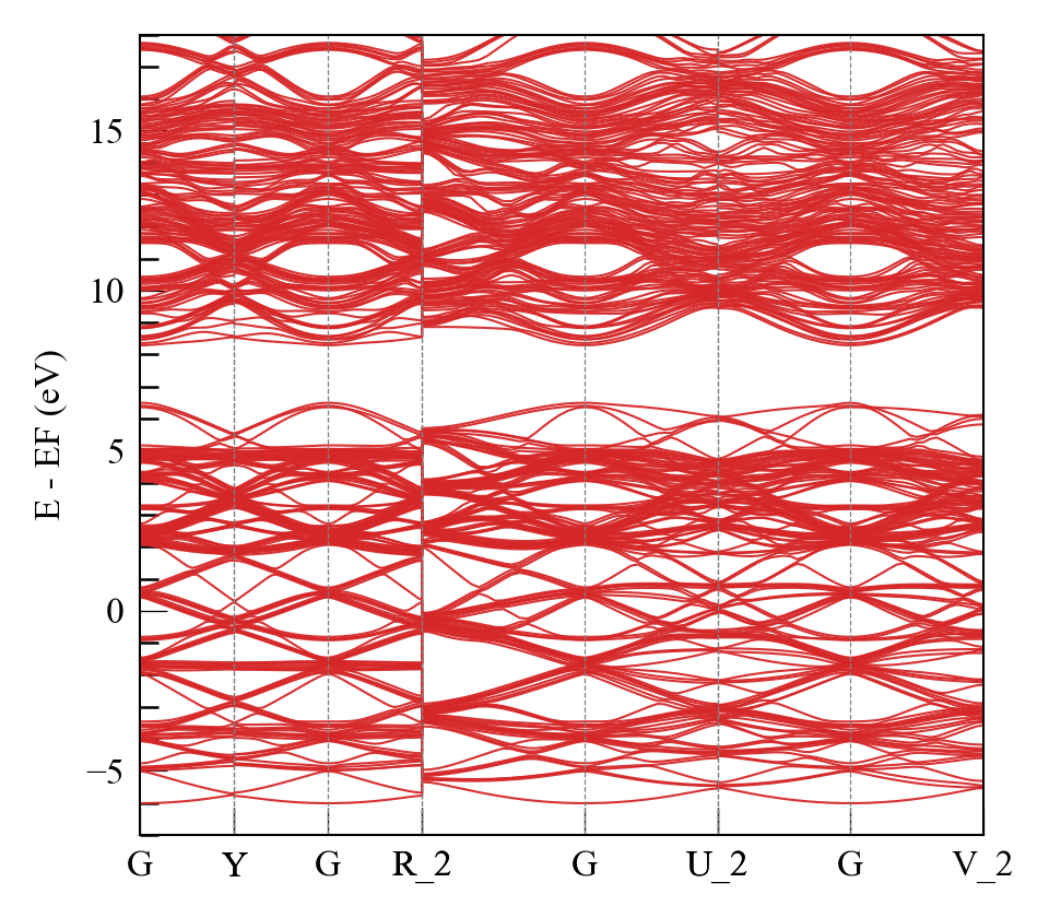
By modify the checkpoint path in the script plot_band.py and running it, the band structure can be obtained in ./band_plot:

python plot_band.py

or just using the command line

dptb run ./band.json -i ./e3_silicon/checkpoint/nnenv.best.pth -o ./band_plot

Now you know how to train a DeePTB-E3 model for Hamiltonian and overlap matrix. For better usage, we encourage the user to read the full input parameters for the DeePTB-E3 model. Also, the DeePTB model supports several post-process tools, and the user can directly extract any predicted properties just using a few lines of code. Please see the basis_api for details.