DeePTB-SK: h-BN#
DeePTB is a package that utilizes machine-learning method to train TB models for target systems with the DFT training data. Here, h-BN monolayer has been chosen as a quick start example.
hBN is a binary compound made of equal numbers of boron (B) and nitrogen (N), we present this as a quick hands-on example. The prepared files are located in:
deeptb/examples/hBN/
├── data
│   ├── kpath.0
│   │   ├── eigenvalues.npy
│   │   ├── info.json
│   │   ├── kpoints.npy
│   │   └── xdat.traj
│   └── struct.vasp
├── input
│   ├── input_first.json
│   ├── input_condband.json
│   ├── input_strain.json
│   ├── input_push_rs.json
|   ├── input_push_w.json
│   └── input_final.json
├── run
│   └── band.json
├── input_short.json
├── ref_ckpts/
├── band_plot/
├── band_plot.py
└── band_plot.ipynb
The input_short.json file contains the least number of parameters that are required to start training the DeePTB model. data folder contains the bandstructure data kpath.0, where another important configuration file info.json is located. input folder contains the input files for different training stages. run folder contains the json for plotting the bandstructure. The ref_ckpts folder contains the reference checkpoints for the model at different training stages. The band_plot folder contains the bandstructure plot. The band_plot.py and band_plot.ipynb is the script for plotting the bandstructure.
First we need to specify the maximum cutoff in building the AtomicData graph in info.json. Here, we set the r_max large enough to contain the 3rd neighbour. This can be assisted by running dptb bond command:
cd deeptb/examples/hBN/data
# to see the bond length
dptb bond struct.vasp
# output:
Bond Type         1         2         3         4         5
------------------------------------------------------------------------
       N-N      2.50      4.34      5.01
       N-B      1.45      2.89      3.82      5.21      5.78
       B-B      2.50      4.34      5.01
Having the data file and input parameter, we can start training our first DeePTB model from scratch. The first step using the parameters defined in input_short.json and we list some important parameters:
 "common_options": {
            "basis": {
                "B": ["2s", "2p"],
                "N": ["2s", "2p"]
            },
            "device": "cpu",
            "dtype": "float32",
            "overlap": false,
            "seed": 120478
    }

"model_options": {
    "nnsk": {
            "onsite": {"method": "none"},
            "hopping": {"method": "powerlaw", "rs":1.6, "w":0.3},
            "soc":{},
            "freeze": false,
            "push":false
        }
    }
We are training a DeePTB model using Slater-Kohster parameterization, so we need to build the nnsk model here. The method of onsite is set to none, which means we do not use onsite correction. The rs of hopping is set to 1.6 which means we use the 1st nearest neighbour for building hopping integrals for now. The basis for each element is set to 2s and 2p which means we use \(2s\) and \(2p\) orbitals as basis.
Since we are using only the valence orbitals at this stage, we can limit the energy window for training in the dataset configuration file info.json as the follwing:
    "bandinfo": {
        "band_min": 0,
        "band_max": 6,
        "emin": null,
        "emax": null
    }
Using the follwing command and we can train the first model:
cd deeptb/examples/hBN
dptb train ./input/input_first.json -o ./first
Here -o indicate the output directory. During the fitting procedure, we can see the loss curve of hBN is decrease consistently. When finished, we get the fitting results in folders first.
By modify the checkpoint path in the script plot_band.py and running it, the band structure can be obtained in ./band_plot:
python plot_band.py
or just using the command line
dptb run ./run/band.json -i ./first/checkpoint/nnsk.best.pth -o ./band_plot
Note: the
basissetting in the plotting script must be the same as in the input.
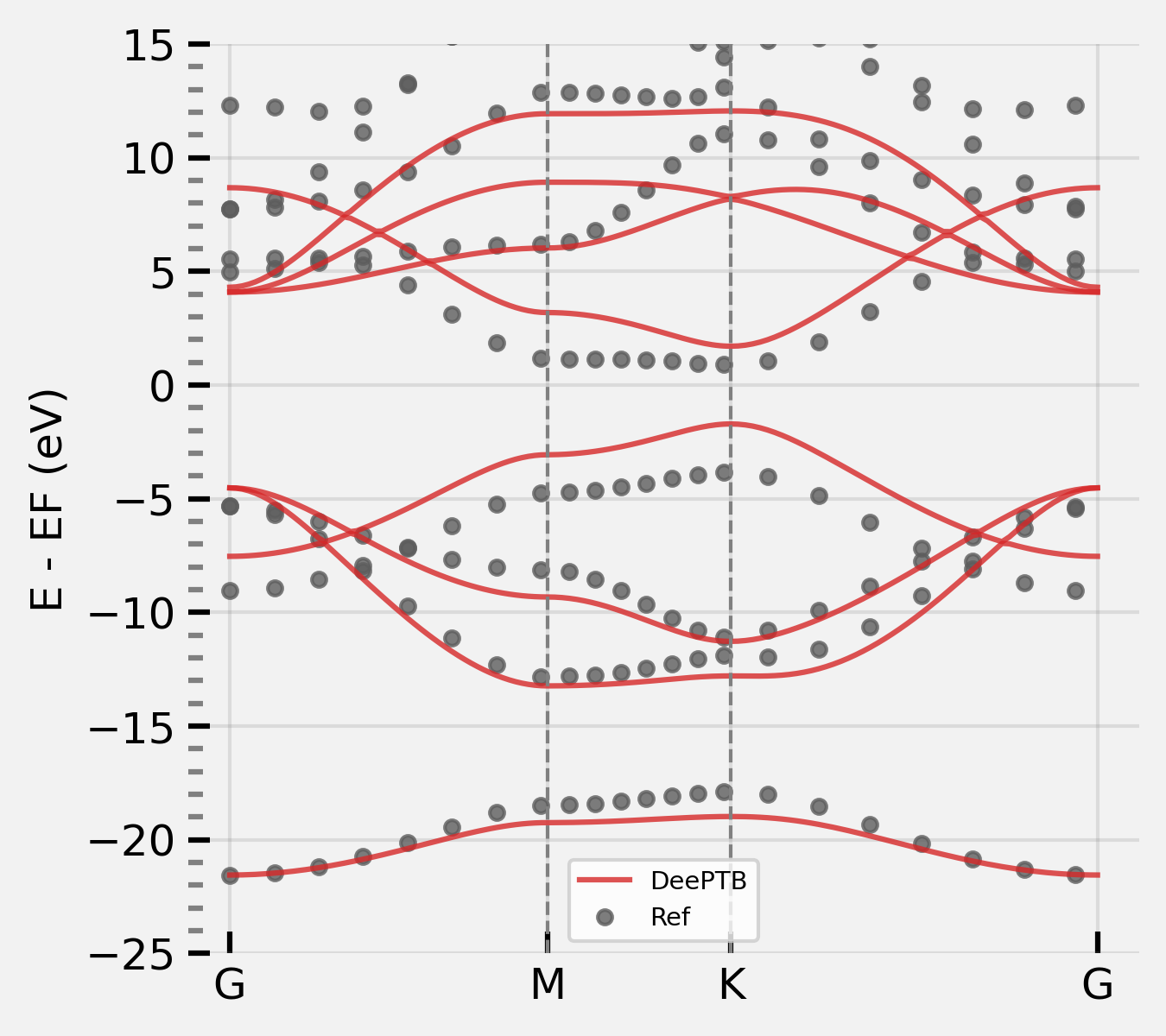
It shows that the fitting has learned the rough shape of the valence bandstructure. To fit the conduction bandstructure, we need to add extra polarized orbitals to the atoms. The polarized orbitals can be added in the input.json by modifying the basis setting:
    "basis": {
        "B": ["2s", "2p", "d*"],
        "N": ["2s", "2p", "d*"]
        }
To train the conduction band, the energy window we previously set in info.json can now be discarded by setting emin and emax to null.
    "bandinfo": {
        "band_min": 0,
        "band_max": 6,
        "emin": null,
        "emax": null
    }
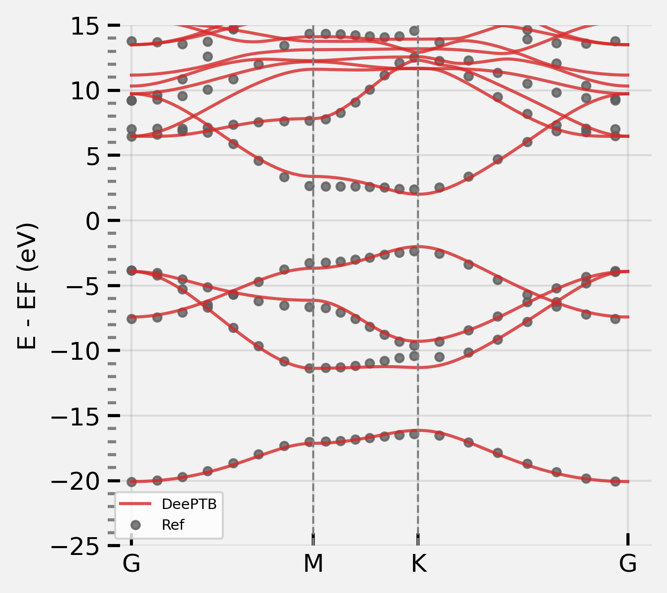
We can then start the training using the previous model and modified input:
dptb train input/input_condband.json -i ./first/checkpoint/nnsk.ep500.pth -o ./condband
-i states initialize the model from the checkpoint file, where the previous model is provided.
The modified input files are provided in
./inputsas references.
After the training is finished, you can get the result in condband folder.
After training, we can plot the bandstructure again using the script:
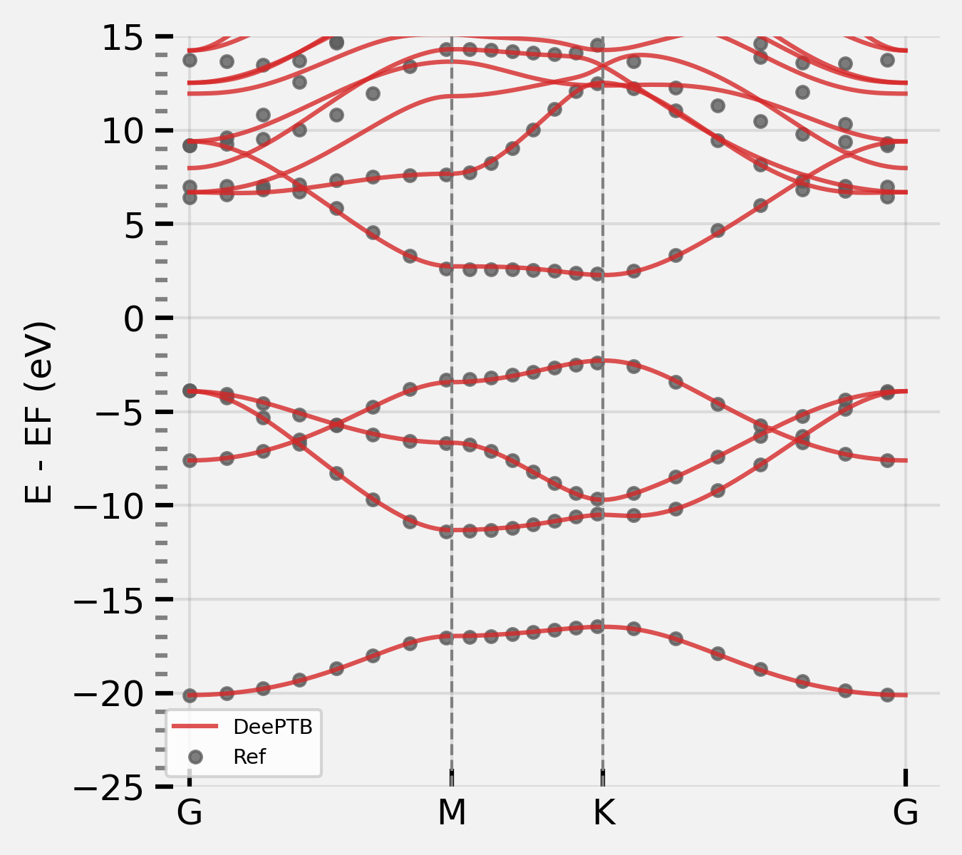
We can further improve the accuracy by incorporating more features of our code, for example, the onsite correction. There are two kinds of onsite correction supported: uniform or strain. We use strain for now to see the effect. Now change the input_short.json by the parameters:
    "model_options": {
        "nnsk": {
            "onsite": {"method": "strain", "rs":1.6, "w":0.3},
            "hopping": {"method": "powerlaw", "rs":1.6, "w": 0.3},
            "freeze": false
        }
    }
After setting we can run the training for strain model:
dptb train input/input_strain.json -i ./condband/checkpoint/nnsk.ep500.pth -o ./strain
We can also plot the band structure of the strain model:
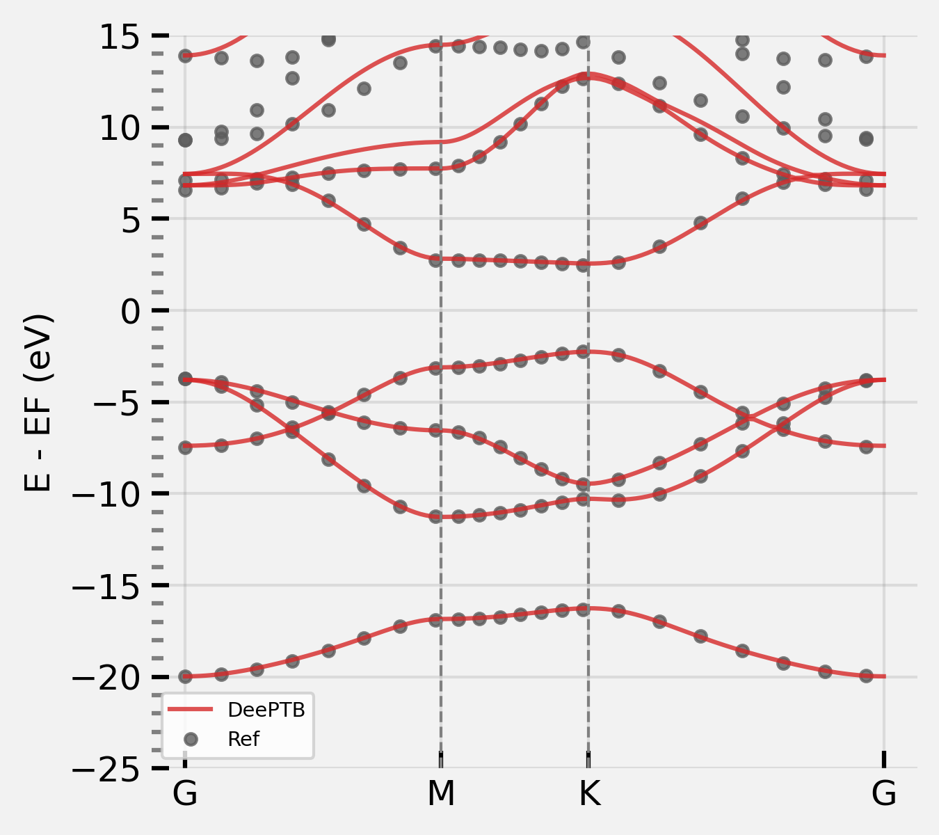
It looks ok, we can further improve the accuracy by adding more neighbours, and training for a longer time. We can gradually increase the decay function cutoff rs from 1st to 3rd neighbour. This can be done by changing the model_options in the input_short.json as follow:
    "model_options": {
        "nnsk": {
            "onsite": {"method": "strain", "rs":1.6, "w":0.3},
            "hopping": {"method": "powerlaw", "rs":1.6, "w": 0.3},
            "soc":{},
            "push": {"rs_thr": 0.02, "period": 10},
            "freeze": false
        }
    }
This means that we gradually add up the rs in decay function, pushing up to 3rd nearest neighbour for considering in calculating bonding. see the input file hBN/input/input_push_rs.json for detail. Then we can run the training again:
dptb train input/input_push_rs.json -i ./strain/checkpoint/nnsk.ep500.pth -o ./push_rs
We finally get the model with more neighbors. We can plot the result again:
we can further push the decay w to 0.2 and train the model again. modify the model options:
    "model_options": {
        "nnsk": {
            "onsite": {"method": "strain", "rs":1.6, "w":0.3},
            "hopping": {"method": "powerlaw", "rs":3.4, "w": 0.3},
            "soc":{},
            "push": {"w_thr": -0.001, "period": 10},
            "freeze": false
        }
    }
note: we change the hopping cutoff rs to 3.4, and the push w_thr to -0.001.
see the input file hBN/input/input_push_w.json and run the training:
dptb train input/input_push_w.json -i ./push_rs/checkpoint/nnsk.iter_rs3.400_w0.300.pth -o ./push_w
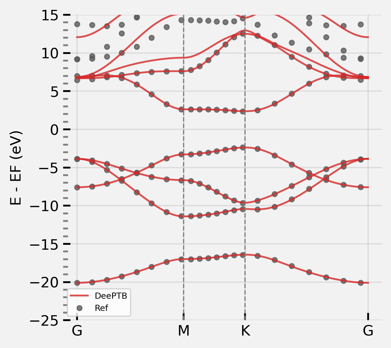
We can the plot the band structure again:
We can again increase more training epochs, using the pushed parameters and turn off push tag. see the input file hBN/input/input_final.json and run the training:
    "model_options": {
        "nnsk": {
            "onsite": {"method": "strain", "rs":1.6, "w":0.3},
            "hopping": {"method": "powerlaw", "rs":3.4, "w": 0.2},
            "soc":{},
            "push": false,
            "freeze": false
        }
    }
dptb train input/input_final.json -i ./push_w/checkpoint/nnsk.iter_rs3.400_w0.210.pth -o ./final
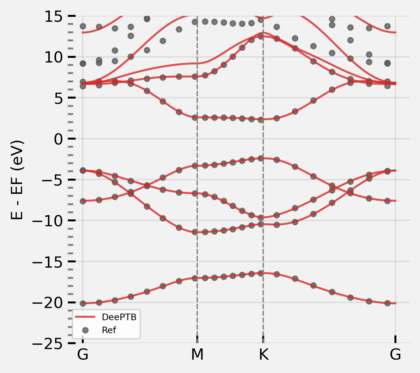
And we can get a fairly good fitting result:
Now you have learned the basis use of DeePTB, however, the advanced functions still need to be explored for accurate and flexible electron structure representation, such as:
environmental correction
spin-orbital interaction
…
Altogether, we can simulate the electronic structure of a crystal system in a dynamic trajectory. DeePTB is capable of handling atom movement, volume change under stress, SOC effect and can use DFT eigenvalues with different orbitals and xc functionals as training targets.